TidyTuesday Week 7/2020: City vs. Resort Hotel

By Lukas Steger

February 23, 2020

A bit late to the party but here it is: My contibution to week 7 #TidyTuesday.
This week’s dataset is about hotel booking demand for two hotels located in Portugal published by Antonio, Almeida and Nunes, 2019. I would like to focus on visualizations and analysis between the two hotels: The city hotel is located in Lisbon, while the resort hotel is located in the region of Algarve.

hotels %>%
  ggplot(aes(x=hotel, fill=hotel))+
  geom_bar()+
  labs(title = "Bookings in the dataset per hotel (Arrival date: 01.07.2015 - 31.08.2017)",
       x= NULL,
       y= "Number of Bookings")+
  guides(fill=FALSE)+
  theme_minimal()+
  theme(plot.background = element_rect(fill = "#F4F4F4"))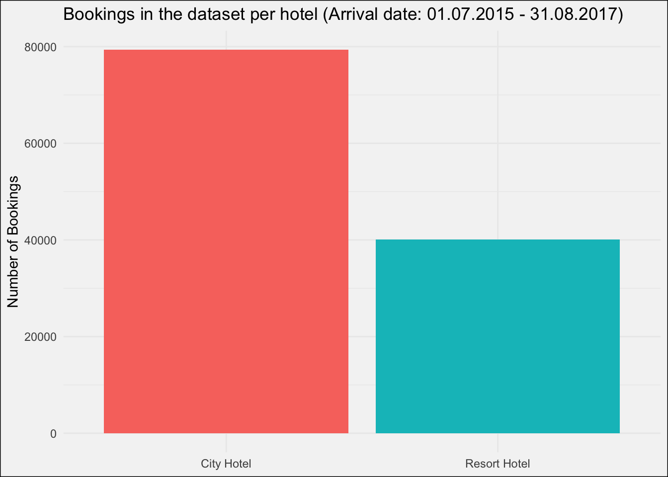

There are almost twice as many bookings in the dataset for the city hotel as for the resort hotel.
The first thing I’m interested in is, how the utilization varies for each hotel throughout the year. The data source does not give any information regarding the maximum capacity for any of the hotels. In a first step I will try to get that information from the data. Some assumptions are made:

Each hotel hits at some point of the observed timeframe their maximum capacity
No-Shows only affect the planned arrival date’s bookings –> booked rooms are allocated to new guests after the first night
Babies are in cluded in the number of beds by adults per booking
Children have their own beds
Bookings with same arrival and check-out date are errors in the data and excluded (680 bookings)

#calculating the stay duration and data cleaning
days_duration <- hotels %>% 
  dplyr::filter(reservation_status != "Canceled") %>%
  select(hotel, date, adults, children, reservation_status, reservation_status_date, stays_in_week_nights, stays_in_weekend_nights, days_in_waiting_list) %>% 
  mutate(reservation_status_date = ymd(reservation_status_date),
         nights_stay = stays_in_week_nights+stays_in_weekend_nights) %>% 
  select(-stays_in_week_nights, -stays_in_weekend_nights) %>% 
  mutate(nights_stay = ifelse(reservation_status == "No-Show", 1, nights_stay)) %>% #reducing no-shows to one night stays
  filter(nights_stay != 0) %>% #remove 0 days stays
  mutate(check_out_date = date+nights_stay,
         last_night = check_out_date-1) %>% #last night of stay were beds are occupied (at check out date new guest can move in)
  mutate(booking_id = row_number()) #add booking id for unnesting

 days_duration_unnested <- days_duration %>%
  transmute(booking_id = booking_id,
            date = map2(date, last_night,  ~ seq(.x, .y, by = 'day')), #add date sequence for each day of the booking
            beds = adults+children, #calculate number of beds per booking
            nights_stay = nights_stay,
            hotel = hotel) %>%
  unnest(cols = c(date)) #bring table into long format one row per day per booking

After the main data cleaning is done let’s have a look at the summary statistics. The maximum number of beds for the city hotel is higher than for the resort hotel, which makes sense according to the overall number of bookings.

hotels_summary <- days_duration_unnested %>% 
  group_by(hotel, date) %>% 
  summarise(beds_occupied = sum(beds)) %>% 
  ungroup() %>% 
  group_by(hotel) %>% 
  summarise(avg= round(mean(beds_occupied), 2), 
    min=min(beds_occupied), 
    max=max(beds_occupied), 
    SD= round(sd(beds_occupied), 2))

city_hotel_max <- hotels_summary$max[1]
resort_hotel_max <- hotels_summary$max[2]

hotels_summary

## # A tibble: 2 x 5
##   hotel          avg   min   max    SD
##   <chr>        <dbl> <dbl> <dbl> <dbl>
## 1 City Hotel    337.     6   532  132.
## 2 Resort Hotel  300.     4   445  102.

With that information it is now possible to plot the average utilization by week for each hotel.

p_weekly_utilization <- days_duration_unnested %>% 
  group_by(hotel, date) %>%
  mutate(utilization_rate = ifelse(hotel == "City Hotel", sum(beds)/city_hotel_max, sum(beds)/resort_hotel_max)) %>%
  ungroup() %>%
  group_by(hotel, week =isoweek(date)) %>%
  summarise(avg_utilization_rate = mean(utilization_rate)) %>% 
  ggplot(aes(x=week, y=avg_utilization_rate, color = hotel))+
  geom_line(size=1)+
  theme_minimal()+
  theme(plot.background = element_rect(fill = "#F4F4F4"))+
  labs(title = "Weekly average bed utilization",
       x = "Week number",
       y = "Utilization in %",
       color = NULL)+
  scale_y_continuous(labels = scales::percent_format(accuracy = 1))+
  gganimate::transition_reveal(as.numeric(week))

gganimate::animate(p_weekly_utilization, end_pause = 40)

There is not really a big difference in utilization rates per hotel, but it seems like the city hotel manages to fill up better during Easter, while in summer the resort hotel does a better job.
Let’s also have a look how the utilizations evolves across week days:

days_duration_unnested %>% 
  group_by(hotel, date) %>%
  mutate(utilization_rate = ifelse(hotel == "City Hotel", sum(beds)/city_hotel_max, sum(beds)/resort_hotel_max)) %>%
  ungroup() %>%
  group_by(hotel,
           weekday = wday(date, label = T, abbr = F)) %>%
  ggplot(aes(x=weekday, y=utilization_rate, fill = hotel))+
  geom_boxplot()+
  theme_minimal()+
  theme(plot.background = element_rect(fill = "#F4F4F4"))+
  labs(title = "Average bed utilization by weekday",
       x = NULL,
       y = "Utilization in %",
       fill = NULL)+
  scale_y_continuous(labels = scales::percent_format(accuracy = 1))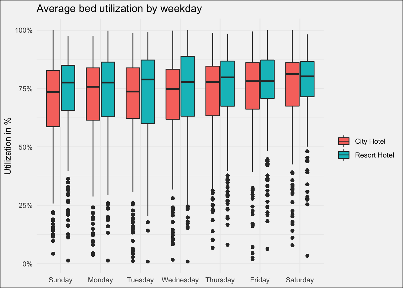

It seems like there is no real difference between the two hotels in terms of utilization by weekday, but it is quite impressive that the mean utilization is around 75%!
Finally, how do the hotels compare in terms of length of stay?

days_duration_unnested %>% 
  group_by(hotel, month=month(date, label = T, abbr = T)) %>%
  summarise(avg_nights = mean(nights_stay)) %>% 
  ggplot(aes(x=month, y=avg_nights, fill = hotel))+
  geom_bar(position="dodge", stat="identity")+
  theme_minimal()+
  theme(plot.background = element_rect(fill = "#F4F4F4"))+
  labs(title = "Average number of nights per booking",
       x = NULL,
       y = "Number of nights",
       fill = NULL)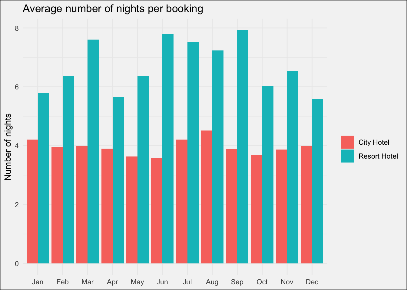

While the stays in the city hotel are relatively stable around 4 nights per booking, the resort hotel has significantly more variance across the year in terms of the number of nights. During the main holiday season around Easter and in the summer months the length of stay raises.

/Lukas