Exploring and predicting cycling rides in Berlin
By Lukas Steger
Introduction
In the year 2015 and 2016 the City of Berlin installed counter stations to monitor cycling rides around the city.
26 of these stations record every cyclists who is passing them. On the website of the Transportation Department the data for the past years is published as an Excel file with hourly counts for each station. This data is the basis for my analysis.
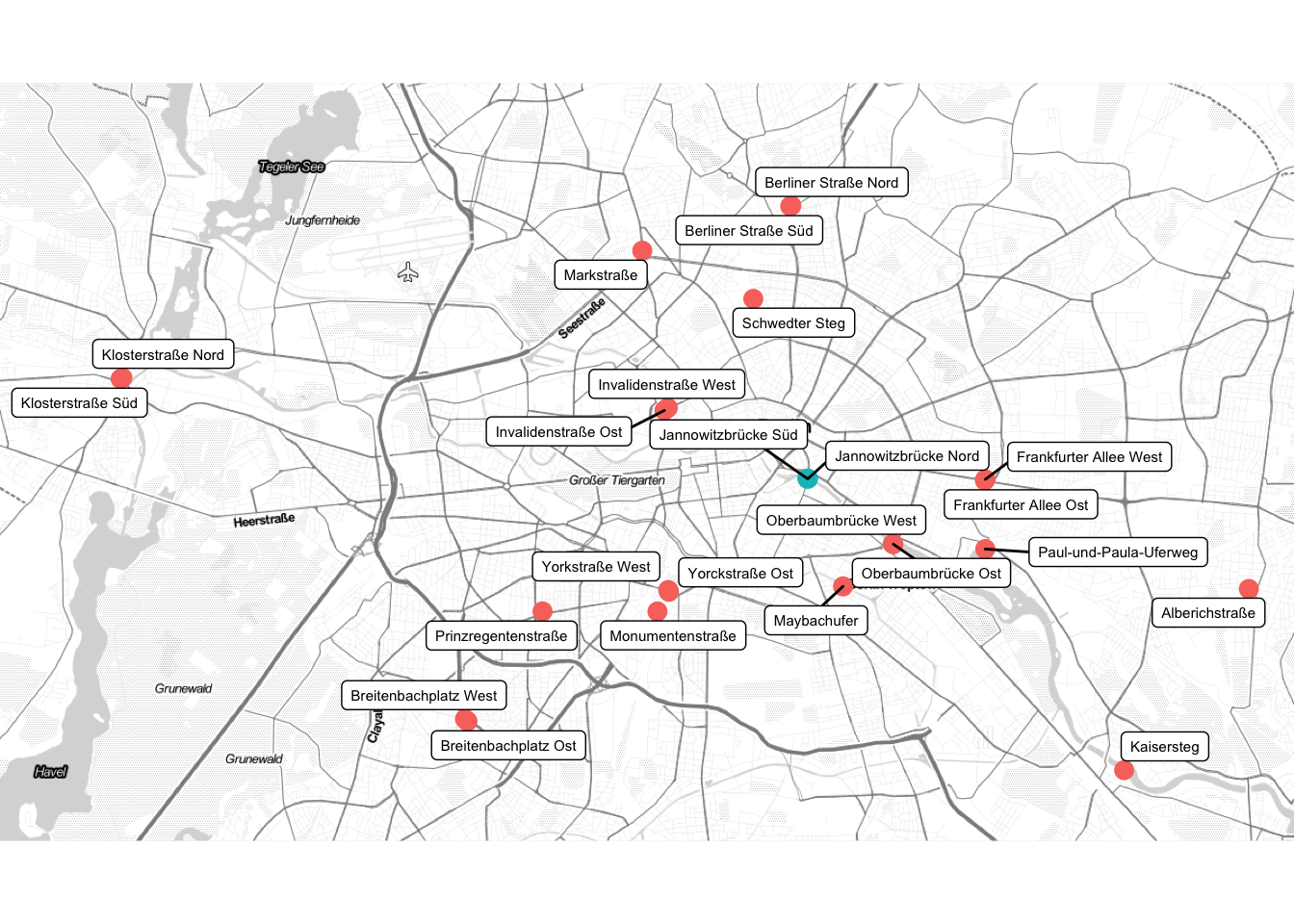
Most of the time im soley focusing only on the two stations at the “Jannowitzbrücke”, which are marked in the plot below:
Can it be too hot to cycle?
But let’s firstly look at the cycling traffic in Berlin as a whole. Berlin’s cyclist clearly prefer the summer over the winter. Although it seems like the summer in 2019, with temperatures close to 40°C, didn’t follow this pattern.
Adding more features
Next to seasonal features, such as week or month, it seems like temperature is a good predictor for the number of rides. Before we continue to explore the data further, let’s add above mentioned features to the counts at Jannowitz Brücke.
From the German Meteorological Service (DWD) the following weather variables in hourly format were retrieved:
- Wind Speed
- Cloud Coverage
- Precipitation
- Humidity
- Temperature
Further, to account for public holidays in Berlin, these dates were imported using the “Feiertags-API” from spiketime and then matched against the data of each observation.
Yes it can be too hot! (and there is a Brückentag effect)
With those additional features it’s much easier to see the effect of really hot days. The plot below shows the average daily rides at the Jannowitz Brücke for the daily maximum temperatures (rounded to integers):
It seems like that from temperatures above 32°C the number of cyclists decreases quite dramatically.
So, I already mentioned something about a “Brückentag effect”. What should that be?
In German Brückentag means the day between two holidays/weekend (eg. Thursday is a public holiday, then Friday is a Brückentag).
For a start have a look how a public holiday affects the rides:
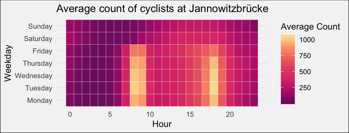
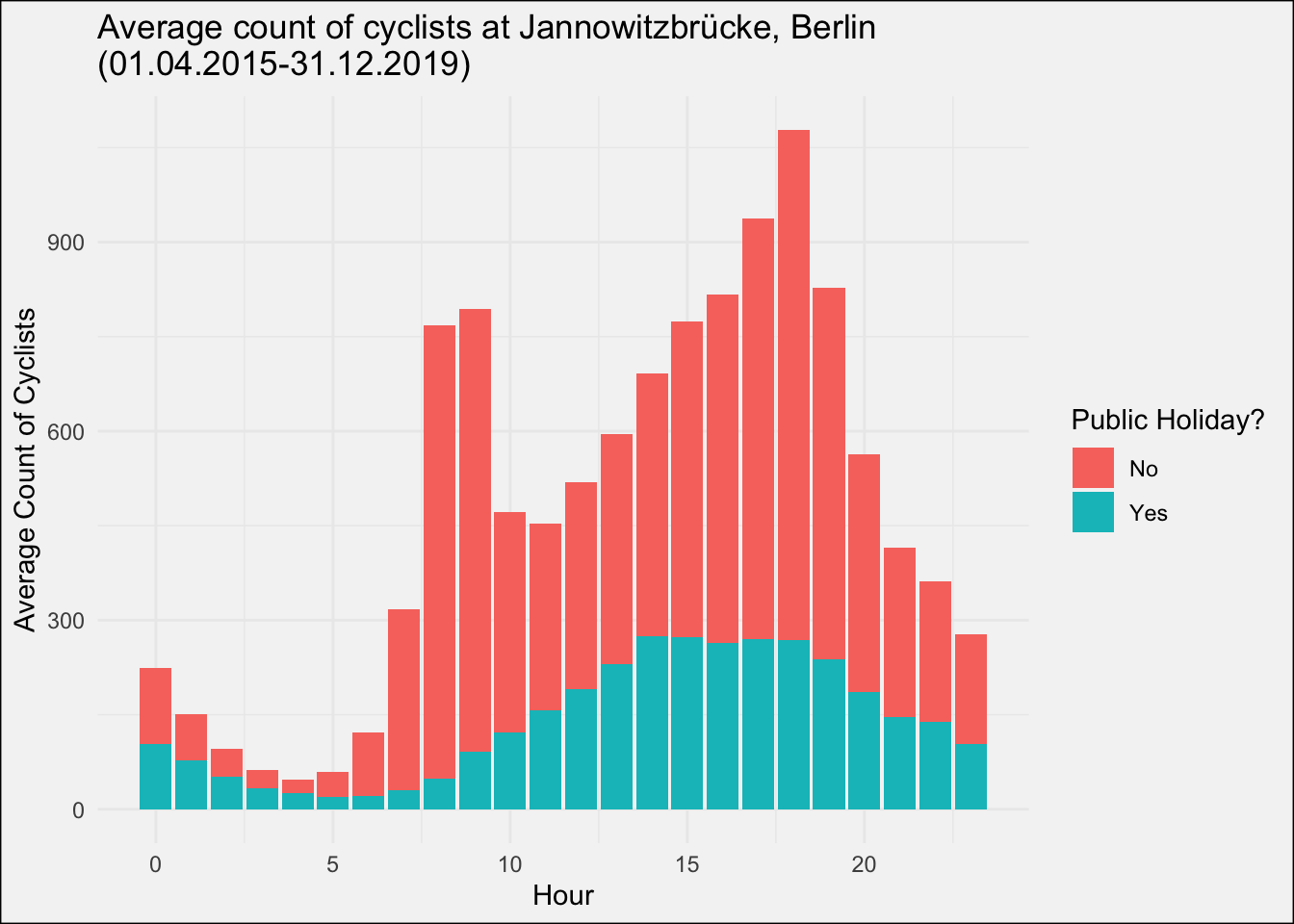 Note how there are two peaks for non-holidays around 8-9 AM and 5-6 PM when people are commuting to and from work. On holidays instead, there is only one wide peak in the afternoon, but all in all on a much lower level.
How does this graph look for Brückentage? 👀
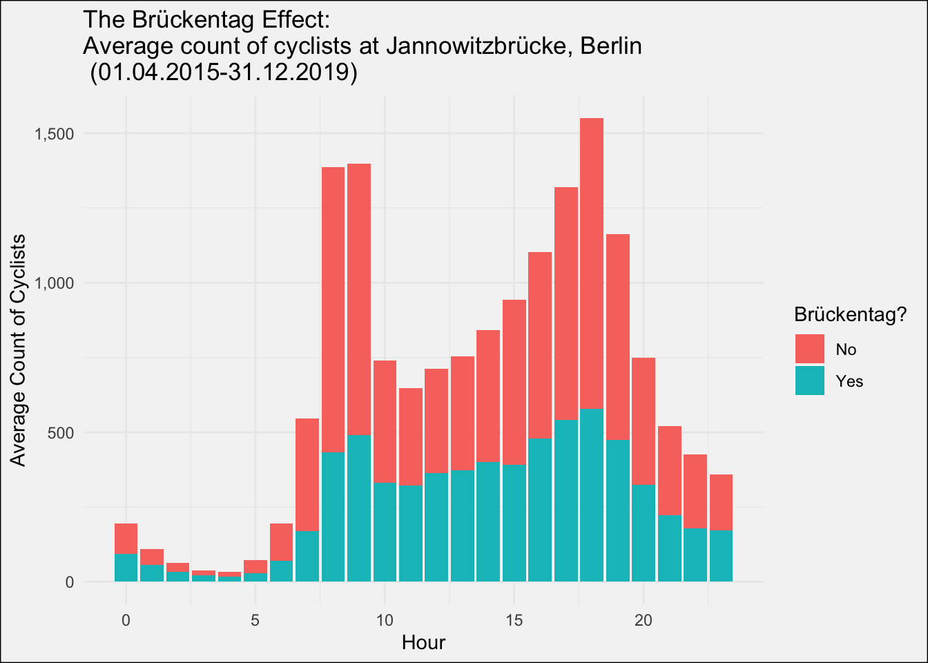
The two commuter peaks are still there, but much weaker. Based on this graphs is seems like roughly 2/3 of the cycle commuters prefer to take a long weekend. 😴
The number of rides varies also quite a lot between the working week and the weekend. Tuesday seems to be the busiest day, while Friday the later peak shifts more towards 4 PM.
Also, note the slight increase in rides Saturday and Sunday morning between 12-3 AM. 🍻 anyone?
Sunday also seems like the day with the least rides in general.
Before starting with the modeling part, let us first inspect the year over year development in cycle rides at Jannowitzbrücke:
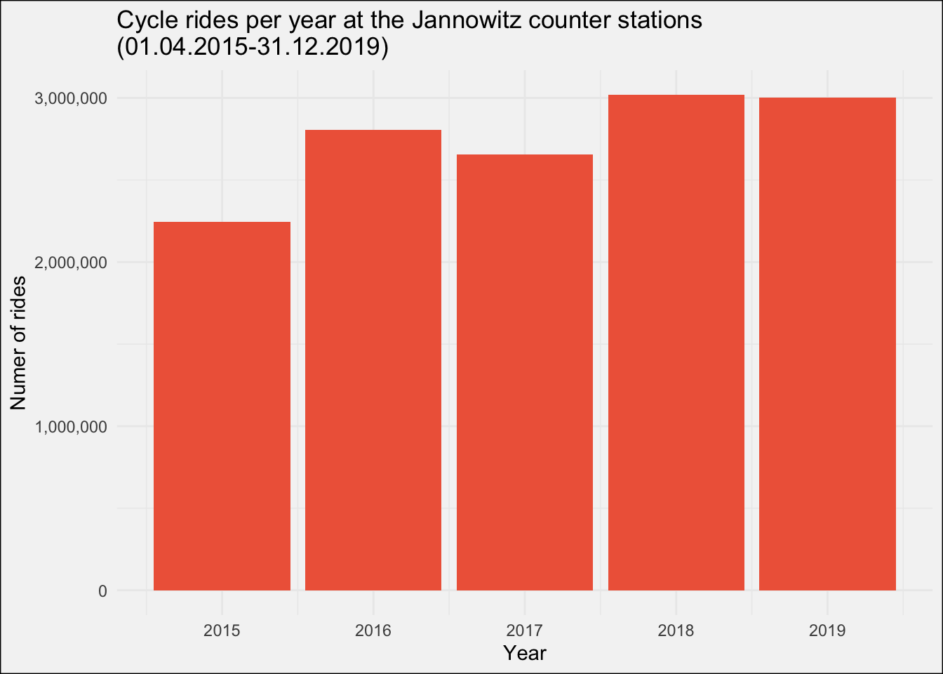
The number of rides seems quite stable (remember the data for 2015 misses January, February and March) over the years, maybe with a slight upwards trend.
As the final step I’m going to inpute a missing value for the count in the dataset and will also add two lagged variables to the dataset as those are usually strong predictors in time series. I decided to take the lag of the last week and last month, which enables us to make predictions with the final model for up to one week in advance (given that we have an accurate 7 day weather forecast..)
#fix missing value in jannowitz_n
combined_raw %>%
  filter(is.na(jannowitz_n)) %>%
  select(date) #missing value on 2019-10-28

#get similar hours (all mondays in october, which are no holiday or brückentag)
october_mondays <- combined_raw %>%
  filter(weekday == 1 & month == 10 & is_holiday == 0 & is_brueckentag == 0 & hour == 4) %>%
  na.omit() %>%
  select(jannowitz_n)

#replace missing value with mean of october mondays at 4am
combined_raw$jannowitz_n[is.na(combined_raw$jannowitz_n)] <- mean(october_mondays$jannowitz_n)


#add lagged variable
combined_raw <- combined_raw %>%
  mutate(lag_last_month = lag(jannowitz_n, n=7*24*4),
         lag_last_week = lag(jannowitz_n, n=7*24))
Modelling with {tidymodels}
{tidymodels} is in a way a successor of {caret} and includes several R packages serving different functions along the modelling process.
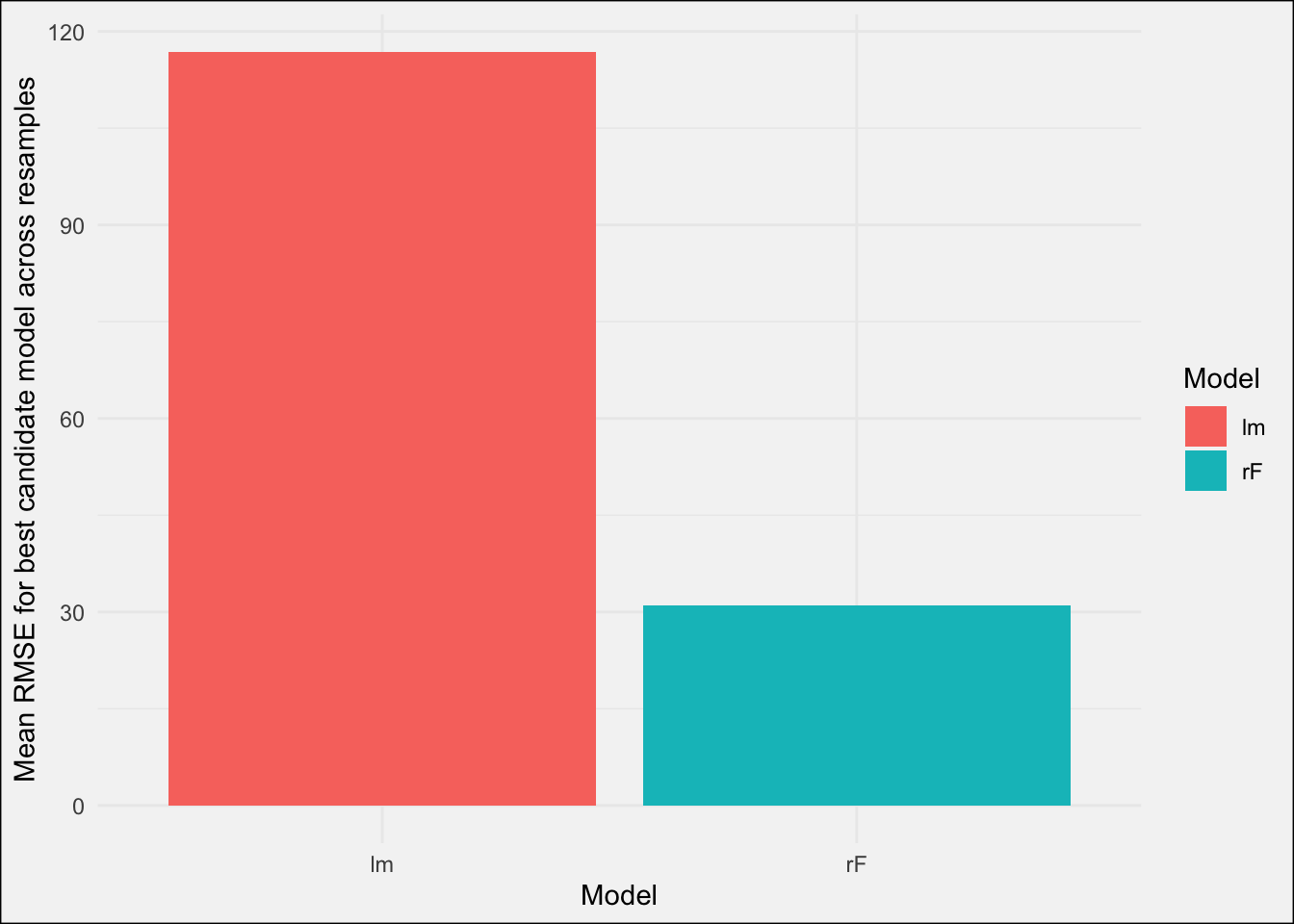
I will use a simple linear regression model (lm) as the baseline and compare it with a random forest model (rF).
The dataset will be splitted into a training set (01-04-2015 to 31-10-2019) and a test set (01-11-2019 to 31-12-2019). Rather than random resamples for cross-validation during tuning the models, rolling_origin() from {rsamples} is used to create 9 resamples (also called slices in the tidymodels world).
train_folds <- rolling_origin(train,
                              initial = 24*365*2, #two years as a moving window
                              assess = 24*7*8, #8 weeks of assessment
                              cumulative = F,
                              skip = 24*7*14) #moving the window by 14 weeks
Starting off, I specify a recipe for each of the models recipe(jannowitz_n ~ ., data = train). jannowitz_n ~ . is the formula for our models and data=train simply tells the recipe where it should look for the data.
Using the %>% operator I sequentially added preprocessing steps to this inital recipe. For the linear regression this looks like the following:
jannowitz_rec_lm <- recipe(jannowitz_n ~ ., data = train) %>%
  step_rm(date) %>%
  step_normalize(starts_with("lag")) %>%
  step_pca(starts_with("lag"),
          num_comp = 1) %>%
  step_num2factor(weekday,
                  levels = c("Mon", "Tue", "Wed", "Thu", "Fri", "Sat", "Sun")) %>%
  step_num2factor(hour,
                  levels = as.character(0:23), transform = function(x) x+1) %>%
  step_num2factor(month,
                  levels = c("Jan", "Feb", "Mar", "Apr", "May", "Jun", "Jul", "Aug", "Sep", "Oct", "Nov", "Dec")) %>%
  step_num2factor(week,
                  levels = as.character(1:53)) %>%
  step_dummy(weekday,
            hour,
            month,
            week,
            one_hot = TRUE) %>%
  step_normalize(all_numeric(),
                -all_outcomes()) %>%
prep()- Removing the date variable as we don’t need it anymore
- normalize the lag variables
- Create a principal component from those two lag variables
- Convert the date related numerical features to a factor
- create dummy variables from these factors
- Normalize all numerical variables (despite the outcome)
- “prep” our recipe on the actual data
In the last step, the recipe looks a the train data and figures out how it would normalize the variables, which variables it actually needs to remove, etc.
After specifying the recipe, I specify the model and its parameters. tune() means, that I don’t tell the model yet exactly which parameter value to use, but rather tune on this parameter. {dials} (another package that is part of tidymodels) comes with a preset range of values for each parameter, which you can access by calling range_get() on the prameter function. (eg. trees() %>% range_get())
For now I didn’t change these preset parameter ranges but if you would like to to that you can do that by providing an lower and upper limit via range_set(c(lower, upper)).
#specify rf model
rf_mod <- rand_forest(mode = "regression",
                      trees = tune(),
                      mtry = tune(),
                      min_n = tune()) %>%
          set_engine(engine = "ranger")

#combine recipe and model specification to one workflow
rf_wflow <- workflow() %>%
  add_recipe(jannowitz_rec_rf) %>%
  add_model(rf_mod)
The final step for the model tuning is to actually fit the candidate model on the resamples via tune_grid() in my case. I only specified that I want a semi-random tuning grid with 25 candidate models via dials::grid_latin_hypercube()). The control argument is similar to the control argument in caret and enables you to turn on verbose mode or to save predictions from all candidate models on all resamples. (watch out, that can be a lot of data!)
set.seed(456321)
initial_rf <- tune_grid(rf_wflow,
                        resamples = train_folds,
                        grid = 25,
                        control = cntrl)
After training the model, the best candidate models including their performance across all resample can be retrieved by calling show_best():
#show best
initial_rf %>%
show_best(metric = "rmse", maximize = FALSE)| mtry | trees | min_n | .metric | .estimator | mean | n | std_err |
|---|---|---|---|---|---|---|---|
| 4 | 488 | 3 | rmse | standard | 30.98 | 9 | 2.78 |
| 13 | 782 | 5 | rmse | standard | 33.70 | 9 | 3.23 |
| 11 | 808 | 6 | rmse | standard | 35.23 | 9 | 3.35 |
| 14 | 1150 | 8 | rmse | standard | 37.91 | 9 | 3.67 |
| 9 | 348 | 14 | rmse | standard | 46.02 | 9 | 4.34 |
Without much surprise the performance in terms of RMSE between the best linear regression model and the best random forest model differs quite significantly across the resamples:
To finalize the best model needs to trained once more on the complete training data:
rf_fitted <- initial_rf %>%
  select_best(metric = "rmse", maximize = FALSE) %>%
  finalize_workflow(x = rf_wflow) %>%
  fit(data=train)
Evaluation on test data
Once that is done, we can use the fitted model to predict on new data with predict(fitted_model, new_data = test). In order to better investigate the model’s errors, I wrote a function to plot the true vs. predicted values of a given fitted model including some time related features such as date, hour or weeknumber:
Clearly the predictions from the random forest look much better than the ones from the linear regression. Main issue with the linear regression are the negative predicted values and in general a more variance.
Although especially the random forest has problems with the last days of the year, where it predicts way over. Maybe a christmas season related variable would help the model here. (‘Last Christmas’ streaming data anyone? 😄)
In addition the values seem a bit skewed for higher counts, where the model under predicts compared to the truth.
I hope you enjoyed this blog post and brief introduction into tidymodels. The full code can be found on my Github.
Thanks for reading!
/Lukas