Using open data to find potential wine shop locations in Germany
By Lukas Steger
Oscar Baruffa started the great initiative of collecting useful resources around R as the Big Book of R. In particular I enjoyed reading and working my way through the book Geocomputation with R by Robin Lovelace, Jakub Nowosad and Jannes Muenchow. In this blog post I would like to adapt their case study in Chapter 13 on Geomarketing from finding potential bike shop locations to wine shops.
Let’s start by loading the required packages:
library(raster)
library(sf)
library(lattice)
library(latticeExtra)
library(grid)
library(gridExtra)
library(classInt)
library(tmap)
library(tidyverse)
library(DataExplorer)
library(revgeo)
library(osmdata)
Next get the last German census data with 1km by 1km raster resolution including demographic information such as population, household size or age. Also I’m going to import the outline of Germany for nicer plotting.
#get german census raster data from 2011
data("census_de", package = "spDataLarge")
force(census_de)
## # A tibble: 361,478 x 13
## Gitter_ID_1km x_mp_1km y_mp_1km Einwohner Frauen_A Alter_D unter18_A ab65_A
## <chr> <int> <int> <int> <int> <int> <int> <int>
## 1 1kmN2684E4334 4334500 2684500 -1 -1 -1 -1 -1
## 2 1kmN2684E4335 4335500 2684500 -1 -1 -1 -1 -1
## 3 1kmN2684E4336 4336500 2684500 -1 -1 -1 -1 -1
## 4 1kmN2684E4337 4337500 2684500 -1 -1 -1 -1 -1
## 5 1kmN2684E4338 4338500 2684500 -1 -1 -1 -1 -1
## 6 1kmN2684E4339 4339500 2684500 -1 -1 -1 -1 -1
## 7 1kmN2685E4334 4334500 2685500 -1 -1 -1 -1 -1
## 8 1kmN2685E4335 4335500 2685500 -1 -1 -1 -1 -1
## 9 1kmN2685E4336 4336500 2685500 -1 -1 -1 -1 -1
## 10 1kmN2685E4337 4337500 2685500 -1 -1 -1 -1 -1
## # … with 361,468 more rows, and 5 more variables: Auslaender_A <int>,
## # HHGroesse_D <int>, Leerstandsquote <int>, Wohnfl_Bew_D <int>,
## # Wohnfl_Whg_D <int>#get outline of Germany from raster package
ger_outline <- raster::getData(country = "DEU", level = 0)I’m going to do some data cleaning on the census data and inspect missing values. Roughly 40% of the raster cells have some missing values, but given that we are mainly interested in the dense populated areas this should be fine.
#some cleanup
input <- census_de %>%
  #as_tibble() %>%
  dplyr::select(x = x_mp_1km,
         y = y_mp_1km,
         pop = Einwohner,
         share_women = Frauen_A,
         mean_age = Alter_D,
         hh_size = HHGroesse_D) %>%
  mutate(across(.cols = where(is.integer), .fns = ~case_when(.x %in% c(-1, -9) ~ NA_integer_,
                                                             TRUE ~ .)))
#inspect missing values
plot_missing(input)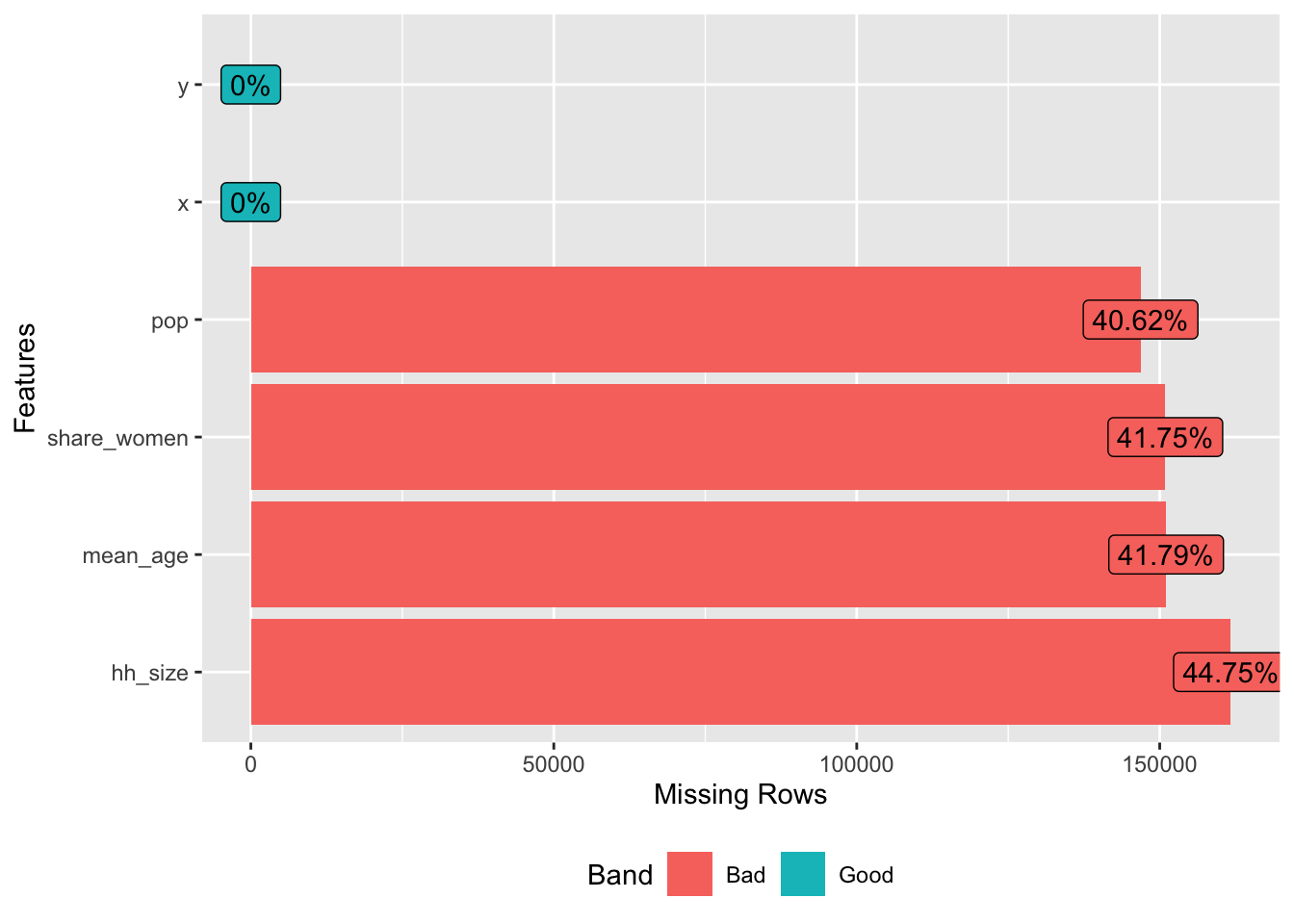
Let’s assume we work for a wine reseller who developed a new store concept that particularly targets young men, as this is an segment the company was struggling with in the past.
To reflect this strategy in the data we are going to reclassify the bins from the census data to assign higher “weights” for the important classes. A overview of the initial bins can be found here.
#create raster
input_ras <- rasterFromXYZ(input, crs = st_crs(3035)$proj4string)
#reproject Germany outline
ger_outline <- spTransform(ger_outline, proj4string(input_ras))

#we are interested in dense populated areas
rcl_pop = matrix(c(1, 1, 127, 2, 2, 375, 3, 3, 1250,
                   4, 4, 3000, 5, 5, 6000, 6, 6, 8000),
                 ncol = 3, byrow = TRUE)
#our store concept particularly targets men
rcl_women = matrix(c(1, 1, 0, 2, 2, 0, 3, 3, 3, 4, 5, 4),
                   ncol = 3, byrow = TRUE)
#which are young
rcl_age = matrix(c(1, 1, 3, 2, 2, 0, 3, 5, 0),
                 ncol = 3, byrow = TRUE)
#and live in smaller households
rcl_hh  = matrix(c(1, 1, 4, 2, 2, 3, 3, 3, 0, 4, 5, 0),
                   ncol = 3, byrow = TRUE)
rcl = list(rcl_pop, rcl_women, rcl_age, rcl_hh)

reclass <- input_ras
for (i in seq_len(nlayers(reclass))) {
  reclass[[i]] = reclassify(x = reclass[[i]], rcl = rcl[[i]], right = NA)
}

#lets plot what we have
reclass_tmap <- tm_shape(reclass)+
  tm_raster(style = "cat", palette = "PuRd", title = "")+
  tm_facets(nrow = 1, free.coords = F, free.scales = T)+
  tm_layout(legend.position = c("left", "top"))
reclass_tmap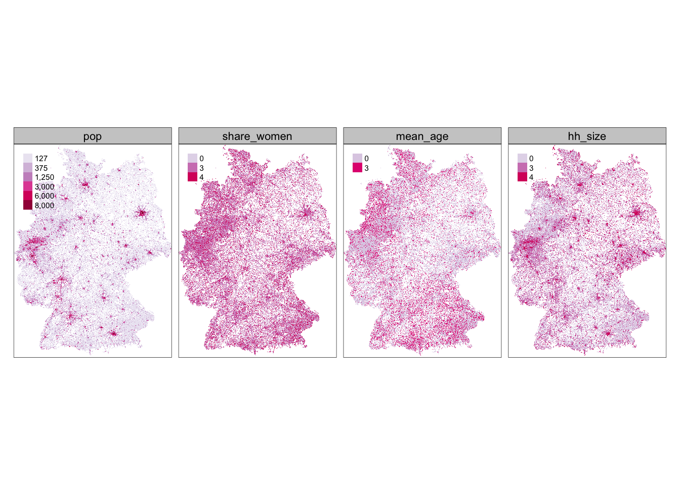
In the next step we change the resolution in order to have bigger rasters (from 1kmx1km to 20kmx20km). Those get filtered to only have rasters where the population is above 400,000 in order to focus only on bigger cities.
#change raster resolution
pop_raster <- raster::subset(reclass, "pop")
names(pop_raster) <- c("pop_raster")
pop <- raster::aggregate(pop_raster, fact = 20, fun = sum)

#only take rasters with more than 400,000 people
pop_agg <- pop[pop > 400000, drop = FALSE]

polys <- pop_agg %>%
  raster::clump() %>%
  rasterToPolygons() %>%
  st_as_sf()

metros <- polys %>%
  group_by(clumps) %>%
  summarize()

metros %>%
  plot()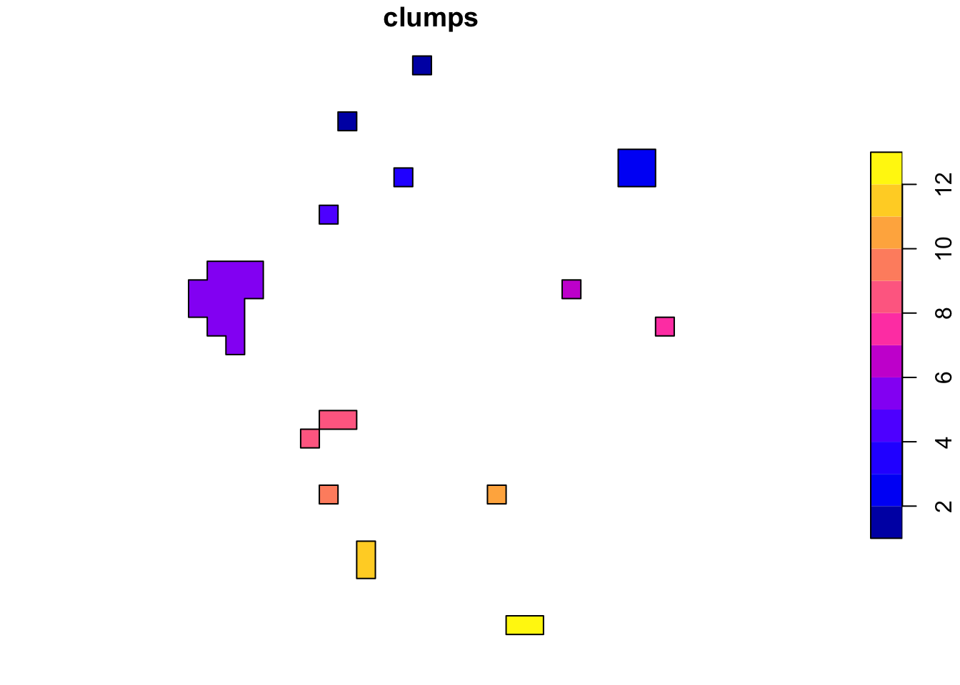
After having defined the areas of interest we get the centroid of each raster and reverse geocode it to extract the city name via the Google Maps API. This is done to have a better understanding which area we are focusing on and the city names will also be the inputs when querying the Overpass API to get OpenStreetMap features in the next step.
metros_wgs <- st_transform(metros, 4326)

coords_with_names <- st_centroid(metros_wgs) %>%
  st_coordinates() %>%
  round(4) %>%
  as_tibble() %>%
  mutate(metro_names = purrr::map2(.x = X, .y=Y, .f = (~revgeo(.x, .y, output = "frame", provider = 'google', API = keyring::key_get("GMAPS_KEY")) %>% select(city)) %>% slowly(rate = rate_delay(pause = 0.2)))) %>%
  unnest(metro_names, keep_empty = TRUE) %>%
  #replace some wrong encodings due to centroids
  mutate(city = case_when(city == "Weyhe" ~ "Bremen",
                          city == "Langenhagen" ~ "Hannover",
                          city %in% c("Wülfrath", "Mettmann") ~ "Duesseldorf",
                          city == "Bannewitz" ~ "Dresden",
                          city == "Eppelheim" ~ "Mannheim",
                          TRUE ~ city))
## [1] "Getting geocode data from Google: https://maps.googleapis.com/maps/api/geocode/json?latlng=53.5457,10&key=AIzaSyC_-FfwRlqJPL5XLaW9-fILaTRQ7s6GPXI"
## [1] "Getting geocode data from Google: https://maps.googleapis.com/maps/api/geocode/json?latlng=53.0006,8.8084&key=AIzaSyC_-FfwRlqJPL5XLaW9-fILaTRQ7s6GPXI"
## [1] "Getting geocode data from Google: https://maps.googleapis.com/maps/api/geocode/json?latlng=52.5091,13.3889&key=AIzaSyC_-FfwRlqJPL5XLaW9-fILaTRQ7s6GPXI"
## [1] "Getting geocode data from Google: https://maps.googleapis.com/maps/api/geocode/json?latlng=52.4669,9.7057&key=AIzaSyC_-FfwRlqJPL5XLaW9-fILaTRQ7s6GPXI"
## [1] "Getting geocode data from Google: https://maps.googleapis.com/maps/api/geocode/json?latlng=52.0988,8.5406&key=AIzaSyC_-FfwRlqJPL5XLaW9-fILaTRQ7s6GPXI"
## [1] "Getting geocode data from Google: https://maps.googleapis.com/maps/api/geocode/json?latlng=51.2541,7.0023&key=AIzaSyC_-FfwRlqJPL5XLaW9-fILaTRQ7s6GPXI"
## [1] "Getting geocode data from Google: https://maps.googleapis.com/maps/api/geocode/json?latlng=51.3662,12.2978&key=AIzaSyC_-FfwRlqJPL5XLaW9-fILaTRQ7s6GPXI"
## [1] "Getting geocode data from Google: https://maps.googleapis.com/maps/api/geocode/json?latlng=50.9701,13.7032&key=AIzaSyC_-FfwRlqJPL5XLaW9-fILaTRQ7s6GPXI"
## [1] "Getting geocode data from Google: https://maps.googleapis.com/maps/api/geocode/json?latlng=50.0617,8.6042&key=AIzaSyC_-FfwRlqJPL5XLaW9-fILaTRQ7s6GPXI"
## [1] "Getting geocode data from Google: https://maps.googleapis.com/maps/api/geocode/json?latlng=49.4025,8.6224&key=AIzaSyC_-FfwRlqJPL5XLaW9-fILaTRQ7s6GPXI"
## [1] "Getting geocode data from Google: https://maps.googleapis.com/maps/api/geocode/json?latlng=49.4055,11.1021&key=AIzaSyC_-FfwRlqJPL5XLaW9-fILaTRQ7s6GPXI"
## [1] "Getting geocode data from Google: https://maps.googleapis.com/maps/api/geocode/json?latlng=48.7784,9.1839&key=AIzaSyC_-FfwRlqJPL5XLaW9-fILaTRQ7s6GPXI"
## [1] "Getting geocode data from Google: https://maps.googleapis.com/maps/api/geocode/json?latlng=48.1415,11.4775&key=AIzaSyC_-FfwRlqJPL5XLaW9-fILaTRQ7s6GPXI"Our company wants to be in close approximately to its competitors and therefore we query OpenStreetMaps for other wine shops in the areas.
#function to combine all results
combine_poi_results <- function(x) {
  # select only specific columns
  result <-  map(x, dplyr::select, osm_id) %>%
    bind_rows()
  return(result)
}

#function to download POI data from osm
collect_pois <- function(x, key, value) {
    message(glue::glue("Downloading {key}s of: "), x, "\n")

    # give the server a bit time
    Sys.sleep(sample(seq(5, 10, 0.1), 1))

    # specify a query with a bounding box and a key
    query = opq(x) %>%
      add_osm_feature(key = key, value = value)

    # Return an OSM query in sf format
    points = osmdata_sf(query)

    # request the same data again if nothing has been downloaded
    iter = 3
    while (nrow(points$osm_points) == 0 & iter > 0) {
      points = osmdata_sf(query)
      iter = iter - 1
    }
    #
    points = st_set_crs(points$osm_points, 4326)
}

shops <- map(coords_with_names %>% pull(city), .f = collect_pois, "shop", "wine")
shops <- combine_poi_results(shops)
After getting the coordinates of wine shop in the next step we count the number of stores per raster and define four classes for an easier interpetation.
shops_trans <- st_transform(shops, proj4string(reclass))
# create wine_shops raster
wine_shops_raster <- rasterize(x = shops_trans, y = reclass, field = "osm_id", fun = "count")

# construct reclassification matrix
fisher_reclassification <- function(raster_obj, layer_name, n_classes = 4) {
  int <-  classInt::classIntervals(values(raster_obj), n = n_classes, style = "fisher")
  int <- round(int$brks)
  rcl <- matrix(c(int[1], rep(int[-c(1, length(int))], each = 2),
                   int[length(int)] + 1), ncol = 2, byrow = TRUE)
  rcl = cbind(rcl, 0:n_classes)
  # reclassify
  raster_obj <- reclassify(raster_obj, rcl = rcl, right = NA)
  names(raster_obj) <- layer_name
  return(raster_obj)
}

wine_shops_rcl <- fisher_reclassification(wine_shops_raster, "wine_shops", 4)
In the last step we add the wine shops as a layer to the census data and filter out all non-dense populated areas as well as areas that have less than 9 points in the scoring model, which essentially simply sums up the classes of our different layers.
# add wine_shops raster
result_layers <- addLayer(reclass, wine_shops_rcl)
# delete population raster
result_layers <- dropLayer(result_layers, "pop")

#final result with equal weights
result <- sum(result_layers, na.rm = TRUE) %>%
  #raster::clump() %>%
  rasterToPolygons()

result_intersection <- result %>%
  st_as_sf() %>%
  st_transform(4326) %>%
  st_intersection(metros_wgs)

cut_off_value <- 9
result_filtered <- result_intersection %>%
  filter(layer >= cut_off_value)

result_intersection %>%
  ggplot(aes(x=layer))+
    geom_density()+
  geom_vline(xintercept = cut_off_value, linetype="dashed")+
    theme_minimal()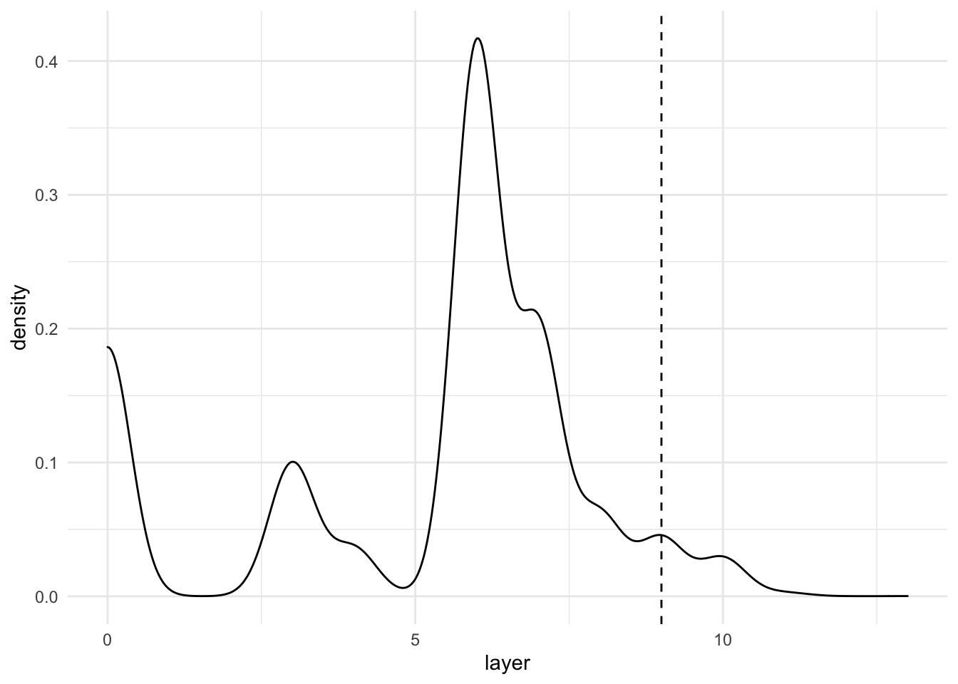
#plot interactive map of results zoomed in on Hamburg and Bremen
tmap_mode("view")
tm_shape(result_filtered)+
tm_fill("layer", palette = sf.colors(5), alpha = .6)+
  tm_view(set.view = c(9.993682, 53.551086, 8))